Differential Privacy and RAPPOR
In 2007 Netflix offered a $1 million prize for a 10% improvement in its recommendation system. They also released a training dataset for the competing developers to train their systems. In order to protect their customer’s privacy, they removed personal information and replaced IDs with random IDs. But Netflix is not the only movie-rating portal out there, there are many others such as IMDb. Researchers linked the Netflix dataset with IMDb to de-anonymize the Netflix dataset using the dates on which an user rated certain movies. This problem isn’t new and remains an important one as today, thanks to computers, we can access larger amounts of data and process them more easily.
In the mid 90s, The Massachusetts Group Insurance Commission (GIC) released anonymized data on state employees that showed every hospital visit. The goal was to help researchers, and the state spent time removing all obvious identifiers such as name, address and Social Security number. A graduate student started hunting for the Governor’s hospital records in the GIC data. She knew that Governor Weld resided in Cambridge, Massachusetts, a city of 54,000 residents and seven ZIP codes. For twenty dollars, she purchased the complete voter rolls from the city of Cambridge. This is a database containing, among other things, the name, address, ZIP code, birth date, and sex of every voter. By combining this data with the GIC records, she found Governor Weld with ease. Only six people in Cambridge shared his birth date, only three of them were men, and of them, only he lived in his ZIP code. The Governor’s health records were de-anonymized.
So, how can we solve this problem? Personal data is already removed from the dataset, and it’s impossible to know whether a dataset can be used to de-anonymize another one. Here is where Differential Privacy appears.
It formalizes the idea that a query should not reveal whether anyone is present in a dataset, much less what their data are. This field was defined by Cynthia Dwork In 2006, using work that started appearing in 2003. It is based on the ideas of randomized response.
Randomized response
Let’s imagine you’re asked “Do you own the attribute A?”, but you don’t want to answer directly. You can use this procedure:
- Throw a coin.
- If head, then answer honestly.
- If tail, then throw the coin again and answer “Yes” if head, “No” if tail.
If the attribute \( A \) is synonymous with illegal behavior, then answering “Yes” is not incriminating
Many responses are significant. Positive responses are given to \( 1/4 \) by people who don’t have the attribute A and \( 3/4 \) by people who possess it
Then we expect to obtain \( (1/4)(1-p) + (3/4)p = (1/4) + p/2 \) positive responses. Hence is possible to estimate p.
If you’re interested in understanding more on how Differential Privacy works, here you can find more information.
Now, the question is, how can we use this technique to collect more complex data?
RAPPOR
RAPPOR is an algorithm developed by Google whose main purpose is to collect data while adding random noise to guarantee Differential Privacy.
Each user is assigned to one of \( m\) cohorts. The value to encode is passed through \( h\) hash functions to encode it into a Bloom filter, and noise is added with probabilities \( p, q, f \).
In RAPPOR, we need to set different parameters:
- Size of the Bloom filter, \( k \): RAPPOR uses a Bloom filter to report the data. When selecting the bloom filter size we should have in mind how many unique values are expected.
- Number of hash functions, \( h \): Bloom filters uses hash functions to encode the values.
- Number of cohorts, \( m \): To avoid collisions, RAPPOR divides the population into different cohorts. This value must be choosen carefully. If it’s too small, collisions are still quite likely, while if it’s too large then each individual cohort provides insufficient signal due to its small sample size.
- Probabilities \( p, q, f \): Noise is added to the Bloom filter with different probabilities. This probabilities determine the level of Differential Privacy along with the number of hash functions used.
Note: This is a very simplified version of RAPPOR, you shouldn’t use it in real life. For optimized implementations, look at the original Google’s repository
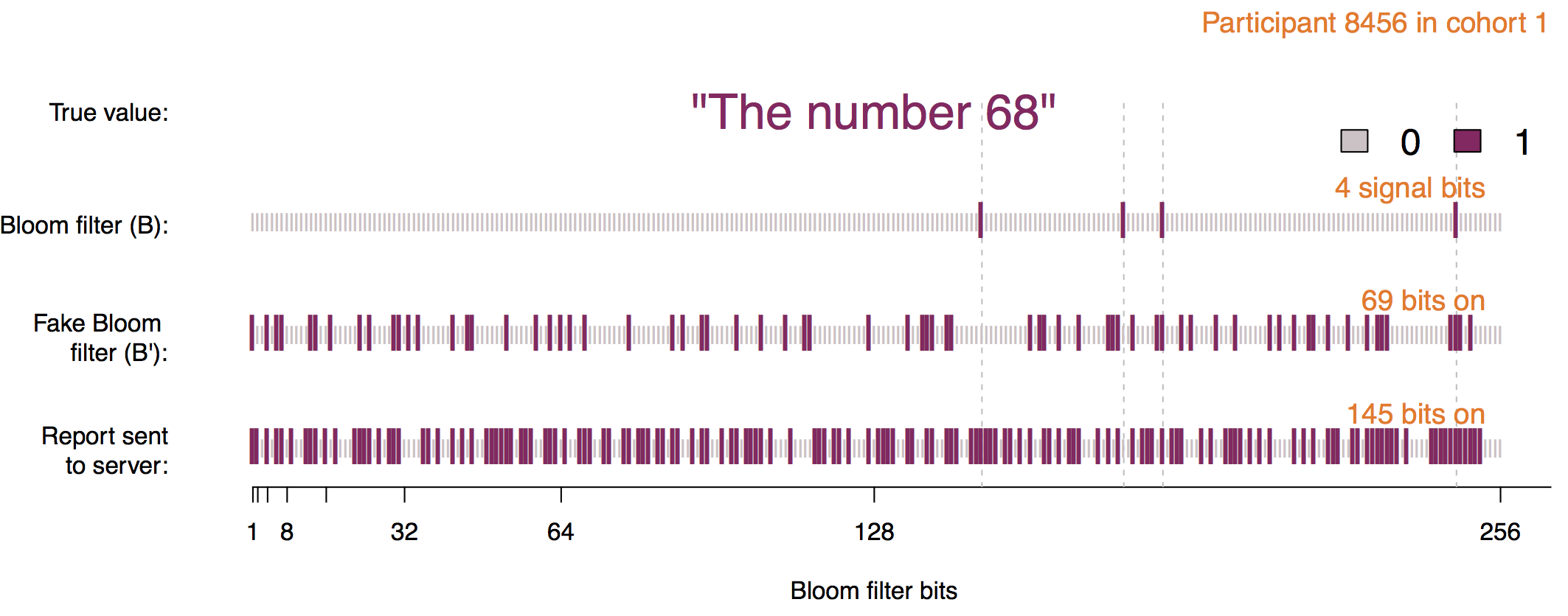
The first step is to encode the original value into the Bloom filter using \( h \) hash functions.
def encode(value, cohort, num_hashes, num_bloombits):
    # create the bloom filter
    bloom = list('0' * num_bloombits)

    # create the hash function to use
    md5 = hashlib.md5(str(cohort) + value)
    digest = md5.digest()
    # get the indexes for encode the original value into the  bloom filter
    idx = [ord(digest[i]) % num_bloombits for i in range(num_hashes)]

    # set the corresponding 'bits' to 1
    for i in idx:
        bloom[i] = '1'
    return bloom
This Bloom filter never leaves the client. The next step is known as Permanent Randomized Response. Here the bits of the Bloom filter are set to 0 or 1 with probability \( f/2 \), or remains unchanged with probability \( 1 - f \). The resulting Bloom filter should be stored in the client and used in the future if the client needs to report the same value more than once.
def get_prr(bloom, prob_f):
    rand = SystemRandom()

    for i in range(len(bloom)):
        val = rand.random()

        if 0 <= val < prob_f / 2:
            bloom[i] = '1'
        elif prob_f / 2 <= val < prob_f:
            bloom[i] = '0'

    return bloom
The Instantaneus Randomize Response is computed using the probabilities \( p \) and \( q \). The resulting Bloom filter will have the bit in position \( i \) set to 1 with probability \( q \) if its value was 1 in the PRR, or with probability \( p \) if its value was 0. The resulting bloom filter is sent for analysis.
def get_irr(bloom, prob_p, prob_q):
    rand = SystemRandom()

    for i in range(len(bloom)):
        prob = prob_p if bloom[i] == '0' else prob_q
        bit = rand.random() < prob

        if bit:
            bloom[i] = '1'

    return bloom
import hashlib
from random import SystemRandom

# params
num_bloombits = 16      # Number of bloom filter bits (k)
num_hashes = 2          # Number of bloom filter hashes (h)
num_cohorts = 64        # Number of cohorts (m)
prob_p = 0.50           # Probability p
prob_q = 0.75           # Probability q
prob_f = 0.50           # Probability f

# original value
value = "v10"

# select cohort
rand = SystemRandom()
cohort = int(rand.random() * num_cohorts)

# encode
original = encode(value, cohort, num_hashes, num_bloombits)

# prr
prr = get_prr(original, prob_f)

# irr
irr = get_irr(prr, prob_p, prob_q)
print ''.join(irr)
RAPPOR analysis
After clients have generated their randomized responses, they send them to a server. This server has the task of aggregating the reports and figuring out which answers were actually given, and how often. To do this, we make use of statistical techniques that are explained in the remainder of this blog post.
The bit arrays are the only information we get from the clients. However, because of the Bloom filter, there are generally infinitely many answers that lead to the same bits being set. This means that we need some set of answers that we explicitely check for. We call this the candidate set. What values are used as candidates is completely dependent on the data that we’re collecting.
Of course we know what bits would be set when hashing these candidate values. If we would also know how often each bit was truly set in the original Bloom filters, before noise was added, then we could model this problem using an equation system. In this system, we’re looking for candidate counts so that the bits set equal the true number of times the individual bits were set. In statistics, this corresponds to a regression problem.
Estimating the counts of bits
Of course, the whole point of differential privacy is that we don’t have access to the originally set bits, so we can’t directly solve this hypothetical equation system. But what we can do is figure out estimates for how often the bits were set. This is possible because we can estimate how much noise was added on average. I won’t go into detail for the exact formulas, as they help little to build intuition, but they can be found in the original RAPPOR paper.
While this approach of making estimates might sound a bit messy, it actually has a fairly good theoretical backing. By the law of large numbers, the estimate will converge to the true counts with an increasing amount of data. This also explains one very important constraint when using differential privacy: We need a lot of users to make sense of the data. The estimates will be very accurate with many users. On the other hand, we can’t control for the random noise well enough if we don’t have a good amount of data.
After having estimated how often bits were changed for the randomized response, we can compute estimates for how often the bits were set in the original Bloom filter. We’ll call these estimates our target vector \( y \). Note that this only gives us information about how often bits were set in total, across all users. We have absolutely no clue about which users had the bits set in their original Bloom filter.
Example
To give a more concrete idea of where we’re going with this, we can stop for a moment and consider this simple example. Let’s say we use a Bloom filter with three bits and two hash functions. After having received the randomized reports from enough users, we estimate the following true bit counts:
- bit 1: 3000
- bit 2: 4000
- bit 3: 1000
We’re collecting data where each client can give exactly one answer out of the possible answers a, b and c. These values correspond to our candidate set. When hashing the candidate values, the following bits would be set:
- a: bits 1, 2 would be set
- b: bits 1, 3 would be set
- c: bits 2, 3 would be set
Given this information, we are looking for counts of how often the answers a, b or c were given so that we arrive at the estimated numbers for the individual bits. The important inside here is that this is an equation system:
- bit 1: count_a + count_b = 3000
- bit 2: count_a + count_c = 4000
- bit 3: count_b + count_c = 1000
Note how this is not just any kind of equation system, it’s a linear equation system. This is great as there are many well-known ways to solve linear equation systems. The straightforward solution for this specific system is that answer a was given 3000 times, b was never given, while c was given 1000 times.
Of course this is a very simple and artificially constructed example, it’s just meant to showcase the problem that the RAPPOR analysis is being reduced to.
Creating the data matrix X
Linear equation systems can generally be well presented using matrices and vectors. We already described out target vector \( y \) earlier. What’s left to talk about is the data matrix \( X \). This matrix encodes what bits are set when candidate values are hashed in different cohorts.
The general idea here is that for each bit and cohort we add a row to the matrix. For each candidate value we add a column. A cell then has value 1 if the corresponding bit would be set when hashing the corresponding candidate value in the respective cohort. Otherwise, it has value 0.
In the above simple example, where we have no cohorts, \( X \) would look like this:
\[X = \begin{bmatrix} 1 & 1 & 0 \\ 1 & 0 & 1 \\ 0 & 1 & 1 \end{bmatrix}\]Now, our linear equation system can be described by \( Xb = y \) where \( b \) gives us the candidate counts that explain the set bits.
Linear regression
All of this is a little bit too simplified. Usually, we can’t directly solve this equation system. One reason is that \( y \) only contains estimates and that our candidate set might be incomplete. This means that the equation system might not have a perfect solution and that we’re generally only looking for an approximate one. However, this is still a fairly standard problem in statistics and is usually solved by fitting a linear regression model.
The other problem is that our system does not entirely consist of linear equations. It wouldn’t make sense to have negative counts. Thus, \( b \) may only contain nonnegative values. This makes the problem a fair bit harder to solve, but again it’s not a completely new problem. There are some implementations of nonnegative least squares (nnls) solvers available that allow us to find the best approximate solution to a linear equation system with the nonnegativity constraint.
Significance tests
It’s worth keeping in mind that we’re only operating on estimates and that some hash collisions are possible. There are many different approximations for the linear equation system and it’s not clear whether candidates with very small counts were actually reported in the original Bloom filters.
All of this screams for statistical significance tests. Computing p-values for linear regression coefficients is a standard practice and is usually done using t-tests. In our case, we use one-sided t-tests because the nonnegativity constraint means that extreme results are only possible in one direction.
We use a significance level of 0.05 to filter out candidate values that don’t have enough evidence for their associated counts. Because there might be a lot of candidate values, we use a Bonferroni corrected significance level. Finally, only the candidate values and frequencies that we have enough confidence in are reported.
Evaluating the results
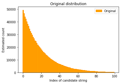
To evaluate how well this works, we can perform a simple simulation. In the simulation shown here, clients report exactly one answer that’s chosen from an exponential distribution.
We can plot this distribution using a bar plot, where the index of possible answers is on the x-axis and their counts are on the y-axis.
The randomization technique is then applied and the randomized reports are analysed by our algorithm. The distribution generated by the algorithm can then be plotted on top of the previous image.
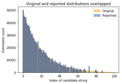
This simulation uses the same parameters that we plan to use in production. As one can see, it works quite well for this original distribution. For the common candidate values, the reported counts are very close to the actual ones. However, it’s not possible to detect candidate values that only occured very few times. There’s just not enough evidence to report them with confidence. Of course only being able to detect common values is not necessarily a bad thing as it means more privacy for users that gave unusual answers.
This post has been written in collaboration with Florian Hartmann